ggplot2::geom_smooth()

Jessica Kramarz

In this document, I will introduce the geom_smooth() function and show what it’s for.

#load ggplot2
library(ggplot2)
#example dataset
library(palmerpenguins)

## Warning: package 'palmerpenguins' was built under R version 4.0.3

data(penguins)

What is it for?

This function helps aid the eye in seeing patterns in the presence of overplotting.

Below we see a plot from the penguins data showing body mass in grams by bill length in mm. Below the plot is not using the geom_smooth() function.

ggplot(penguins, aes(body_mass_g, bill_length_mm)) +
  geom_point() + labs(title="Bill length (mm) vs Body mass (g)") +
  xlab("Body Mass (g)") +
  ylab("Bill Length (mm)")

## Warning: Removed 2 rows containing missing values (geom_point).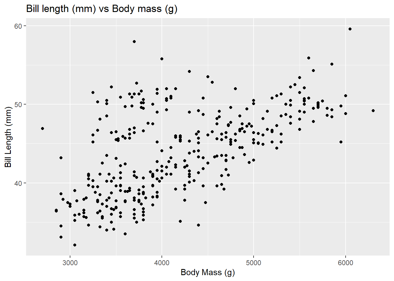

While a general trend can be identified of bill length (mm) increasing with body mass (g), it becomes more clear and easier to identify with the geom_smooth() function included.

ggplot(penguins, aes(body_mass_g, bill_length_mm)) +
  geom_point() +
  geom_smooth() +
    labs(title="Bill length (mm) vs Body mass (g)") +
  xlab("Body Mass (g)") +
  ylab("Bill Length (mm)")

## `geom_smooth()` using method = 'loess' and formula 'y ~ x'

## Warning: Removed 2 rows containing non-finite values (stat_smooth).

## Warning: Removed 2 rows containing missing values (geom_point).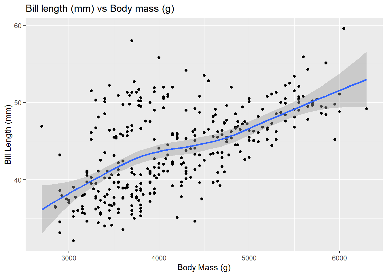

Without specification of method in the argument, the geom_smooth() function will default to loess. Loess is a type of smoothing which is generally done with data that has 1000 observations or less, as it can be time consuming if they exceed 1000. If the observations are greater than 1,000, gam() is the default smoothing method.

Another helpful modeling function to know is geom_smooth(method=“lm”), this creates a straight line or linear fit. This could be helpful when trying to determine if a relationship is linear.

ggplot(penguins, aes(body_mass_g, bill_length_mm)) +
  geom_point() +
  geom_smooth(method='lm') +
    labs(title="Bill length (mm) vs Body mass (g)") +
  xlab("Body Mass (g)") +
  ylab("Bill Length (mm)")

## `geom_smooth()` using formula 'y ~ x'

## Warning: Removed 2 rows containing non-finite values (stat_smooth).

## Warning: Removed 2 rows containing missing values (geom_point).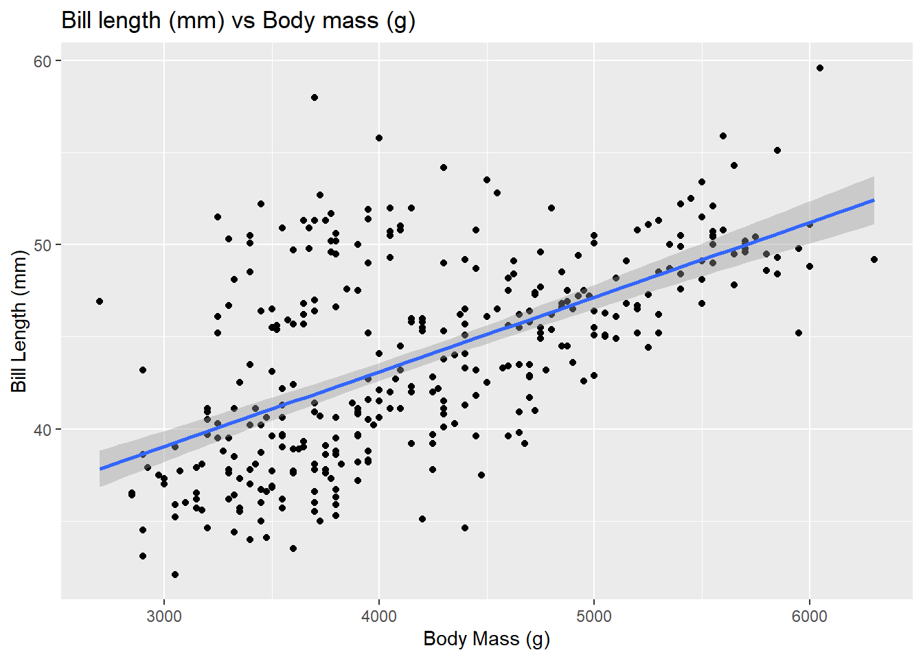

Additionally, without specification of formula in the argument the function will default the formula to ‘y~x’ for smoothing. If you think a quadratic fucntion might be a good approximation for the fit of your data, we can go back in to the linear model and change the formula to include a squared term for x: geom_smooth(method = “lm”, formula = y ~x + I(x^2)). However, for our data, the linear relationship is rather strong.

Also by default, the function will display confidence intervals around the smooth. Since the function is TRUE by default, set se = FALSE, as done below, to remove the confidence intervals.

ggplot(penguins, aes(body_mass_g, bill_length_mm)) +
  geom_point() +
  geom_smooth(se = FALSE) +
    labs(title="Bill length (mm) vs Body mass (g)") +
  xlab("Body Mass (g)") +
  ylab("Bill Length (mm)")

## `geom_smooth()` using method = 'loess' and formula 'y ~ x'

## Warning: Removed 2 rows containing non-finite values (stat_smooth).

## Warning: Removed 2 rows containing missing values (geom_point).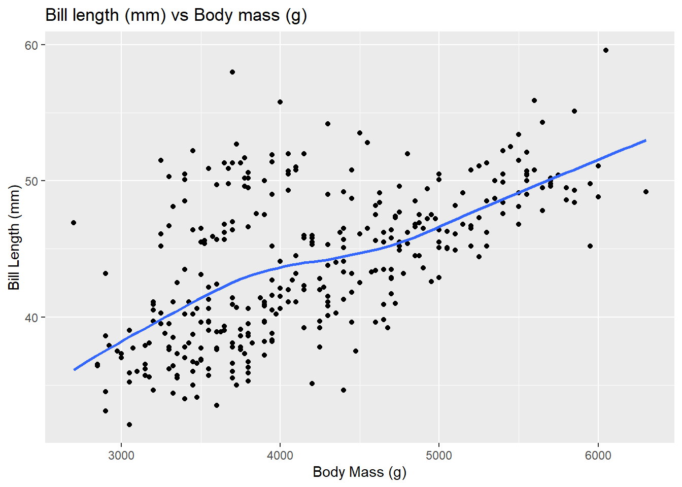

Is it helpful?

This function can be helpful as it can be hard to observe trends with just data points alone. This can be especially helpful when trying to understand regressions.

To learn about more of the functions of geom_smooth() try typing “?geom_smooth” into your R console.