ggplot2::geom_density()

Bradie Winders

In this document, I will introduce the geom_density function and show what it’s for.

#load tidyverse up
library(tidyverse)

## Warning: package 'tidyverse' was built under R version 4.0.3

## -- Attaching packages --------------------------------------- tidyverse 1.3.0 --

## v tibble  3.0.6     v dplyr   1.0.4
## v tidyr   1.1.2     v stringr 1.4.0
## v readr   1.4.0     v forcats 0.5.1
## v purrr   0.3.4

## Warning: package 'tibble' was built under R version 4.0.3

## Warning: package 'tidyr' was built under R version 4.0.3

## Warning: package 'readr' was built under R version 4.0.3

## Warning: package 'purrr' was built under R version 4.0.3

## Warning: package 'dplyr' was built under R version 4.0.3

## Warning: package 'stringr' was built under R version 4.0.3

## Warning: package 'forcats' was built under R version 4.0.3

## -- Conflicts ------------------------------------------ tidyverse_conflicts() --
## x dplyr::filter() masks stats::filter()
## x dplyr::lag()    masks stats::lag()

#example dataset
library(palmerpenguins)

## Warning: package 'palmerpenguins' was built under R version 4.0.3

data(penguins)

What is it for?

geom_density() is a function from the ggplot2 package that creates smooth density estimate plots, which are the smoothed versions of histograms. It is great for visualizing distribution, skewness, and kurtosis of continuous data. Many choose to overlay density plots over histograms with geom_density(), or create multiple density plots from different variables.

glimpse(penguins)

## Rows: 344
## Columns: 8
## $ species           <fct> Adelie, Adelie, Adelie, Adelie, Adelie, Adelie, A...
## $ island            <fct> Torgersen, Torgersen, Torgersen, Torgersen, Torge...
## $ bill_length_mm    <dbl> 39.1, 39.5, 40.3, NA, 36.7, 39.3, 38.9, 39.2, 34....
## $ bill_depth_mm     <dbl> 18.7, 17.4, 18.0, NA, 19.3, 20.6, 17.8, 19.6, 18....
## $ flipper_length_mm <int> 181, 186, 195, NA, 193, 190, 181, 195, 193, 190, ...
## $ body_mass_g       <int> 3750, 3800, 3250, NA, 3450, 3650, 3625, 4675, 347...
## $ sex               <fct> male, female, female, NA, female, male, female, m...
## $ year              <int> 2007, 2007, 2007, 2007, 2007, 2007, 2007, 2007, 2...

ggplot(penguins, aes(body_mass_g, fill=species)) + geom_density(alpha = 0.2) + theme_bw() + xlab("body mass (g)") + ggtitle("Body Mass by Species")

## Warning: Removed 2 rows containing non-finite values (stat_density).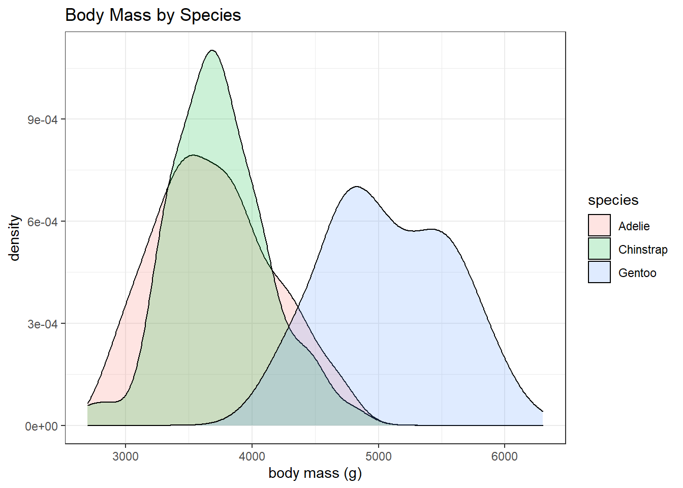

Is it helpful?

It is extremely helpful when performing exploratory data analysis to assess distribution of numerical variables and compare them to each other. Evaluating descriptive statistics of the data go hand-in-hand with visualization to get a better understanding of the story the data tell. This is why geom_density() is a powerful function.