ggplot2::geom_tile()
Lindsay Brown
In this document, I will introduce the geom_tile() function and show what it is for.
#load libraries
library(ggplot2)
## Warning: package 'ggplot2' was built under R version 4.0.3library(tidyverse)## Warning: package 'tidyverse' was built under R version 4.0.3## -- Attaching packages --------------------------------------- tidyverse 1.3.0 --## v tibble 3.0.6 v dplyr 1.0.4
## v tidyr 1.1.2 v stringr 1.4.0
## v readr 1.4.0 v forcats 0.5.1
## v purrr 0.3.4## Warning: package 'tibble' was built under R version 4.0.3## Warning: package 'tidyr' was built under R version 4.0.3## Warning: package 'readr' was built under R version 4.0.3## Warning: package 'purrr' was built under R version 4.0.3## Warning: package 'dplyr' was built under R version 4.0.3## Warning: package 'stringr' was built under R version 4.0.3## Warning: package 'forcats' was built under R version 4.0.3## -- Conflicts ------------------------------------------ tidyverse_conflicts() --
## x dplyr::filter() masks stats::filter()
## x dplyr::lag() masks stats::lag()Data
I used the dataset "Food Consumption and CO2 emissions from the Tidy Tuesday website year 2020. This dataset is rather large, so first we had to create a smaller subset of data for the plot.
#example dataset found from TidyTuesday page.

food_consumption <- readr::read_csv('https://raw.githubusercontent.com/rfordatascience/tidytuesday/master/data/2020/2020-02-18/food_consumption.csv')
##
## -- Column specification --------------------------------------------------------
## cols(
## country = col_character(),
## food_category = col_character(),
## consumption = col_double(),
## co2_emmission = col_double()
## )food_consumption %>% pull(country) %>% unique()## [1] "Argentina" "Australia" "Albania"
## [4] "Iceland" "New Zealand" "USA"
## [7] "Uruguay" "Luxembourg" "Brazil"
## [10] "Kazakhstan" "Sweden" "Bermuda"
## [13] "Denmark" "Finland" "Ireland"
## [16] "Greece" "France" "Canada"
## [19] "Norway" "Hong Kong SAR. China" "French Polynesia"
## [22] "Israel" "Switzerland" "Netherlands"
## [25] "Kuwait" "United Kingdom" "Austria"
## [28] "Oman" "Italy" "Bahamas"
## [31] "Portugal" "Malta" "Armenia"
## [34] "Slovenia" "Chile" "Venezuela"
## [37] "Belgium" "Germany" "Russia"
## [40] "Croatia" "Belarus" "Spain"
## [43] "Paraguay" "New Caledonia" "South Africa"
## [46] "Barbados" "Lithuania" "Turkey"
## [49] "Estonia" "Mexico" "Costa Rica"
## [52] "Bolivia" "Ecuador" "Panama"
## [55] "Czech Republic" "Romania" "Colombia"
## [58] "Maldives" "Cyprus" "Serbia"
## [61] "United Arab Emirates" "Algeria" "Ukraine"
## [64] "Pakistan" "Swaziland" "Latvia"
## [67] "Bosnia and Herzegovina" "Fiji" "South Korea"
## [70] "Poland" "Saudi Arabia" "Botswana"
## [73] "Macedonia" "Hungary" "Trinidad and Tobago"
## [76] "Tunisia" "Egypt" "Mauritius"
## [79] "Bulgaria" "Morocco" "Slovakia"
## [82] "Niger" "Kenya" "Jordan"
## [85] "Japan" "Georgia" "Grenada"
## [88] "El Salvador" "Cuba" "China"
## [91] "Honduras" "Taiwan. ROC" "Angola"
## [94] "Jamaica" "Namibia" "Belize"
## [97] "Malaysia" "Zimbabwe" "Guatemala"
## [100] "Uganda" "Nepal" "Iran"
## [103] "Tanzania" "Senegal" "Peru"
## [106] "Nicaragua" "Vietnam" "Ethiopia"
## [109] "Myanmar" "Congo" "Zambia"
## [112] "Cameroon" "Madagascar" "Malawi"
## [115] "Guinea" "Nigeria" "Rwanda"
## [118] "Philippines" "Ghana" "Togo"
## [121] "Gambia" "India" "Thailand"
## [124] "Mozambique" "Cambodia" "Sierra Leone"
## [127] "Sri Lanka" "Indonesia" "Liberia"
## [130] "Bangladesh"glimpse (food_consumption)## Rows: 1,430
## Columns: 4
## $ country <chr> "Argentina", "Argentina", "Argentina", "Argentina", "...
## $ food_category <chr> "Pork", "Poultry", "Beef", "Lamb & Goat", "Fish", "Eg...
## $ consumption <dbl> 10.51, 38.66, 55.48, 1.56, 4.36, 11.39, 195.08, 103.1...
## $ co2_emmission <dbl> 37.20, 41.53, 1712.00, 54.63, 6.96, 10.46, 277.87, 19...subset_countries <- c("Argentina", "Kazakhstan", "Sweden", "Ireland", "Venezuela", "Egypt", "Indonesia")
food_consumption <- food_consumption %>%
filter(country %in% subset_countries)What is it for?
geom_tile is part of the ggplot2 package that can create heatmaps, a way of looking at 3 dimensional data in 2 dimensions.
for this heatmap we are going to look at the smaller subset of data created above. our axis will be as follows:
x = country
y = food_category
z (“fill”) = consumption
in geom_tile the argument show.legend defaults NA to show a legend if aesthetics such as (x = __ y = __ ) are mapped, however you can set this to FALSE if you do not want a legend, or TRUE if you always want a legend.
ggplot(food_consumption) +
  aes(x=country, y=food_category, fill=consumption) +
  geom_tile() +
  labs(title="consumption of food by category and country") +
  xlab("Country") +
  ylab("Food Category")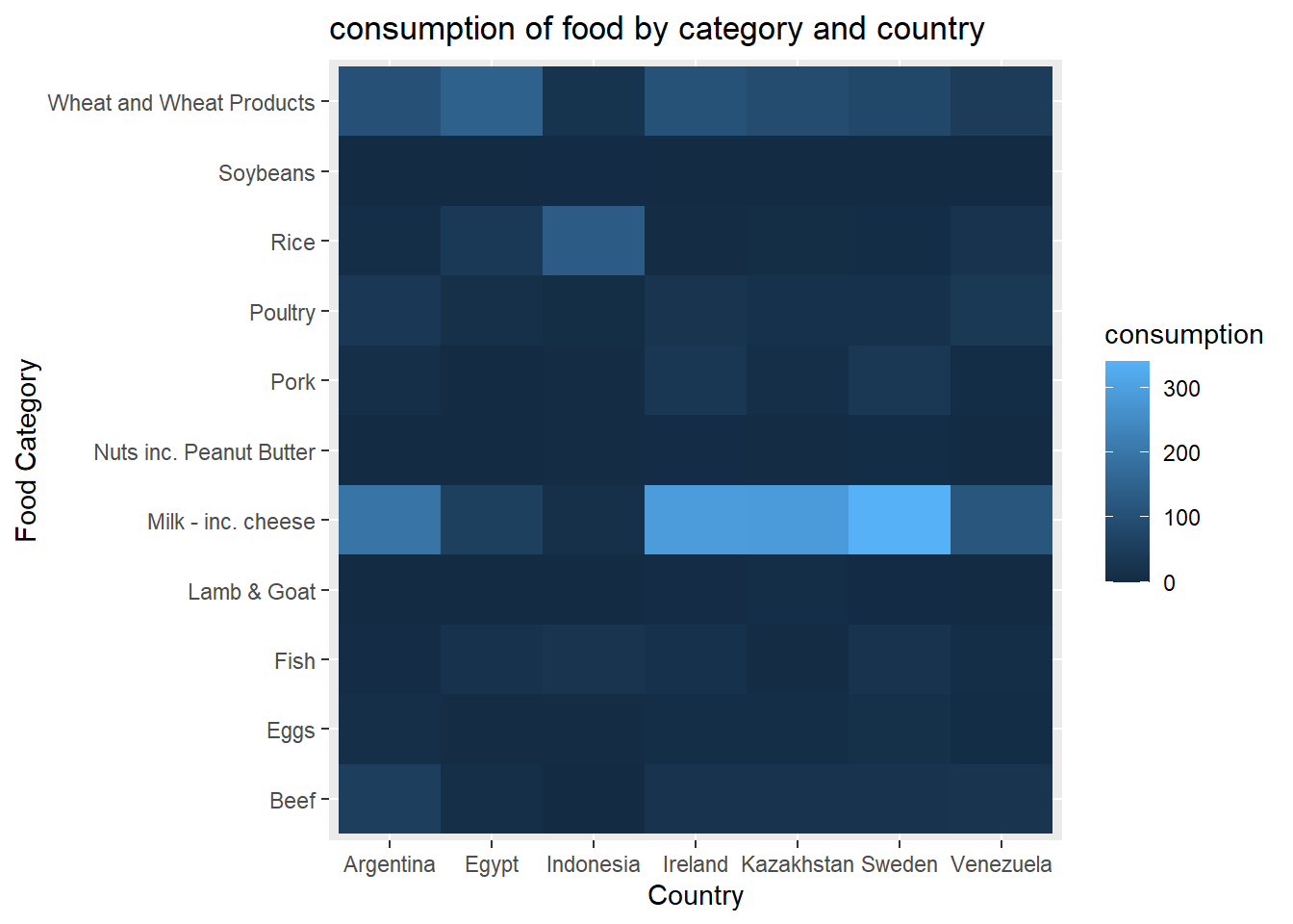
Color
You can use scale_fill_gradient arguments (low = ____ high=____) to customize your color scheme. The default for geom_tile() is the blue that we saw above.
ggplot(food_consumption) +
  aes(x=country, y=food_category, fill=consumption) +
  geom_tile() +
  scale_fill_gradient(
                      low = "#005e49",
                      high = "#91ffe6") +
  labs(title="consumption of food by category and country") +
  xlab("Country") +
  ylab("Food Category")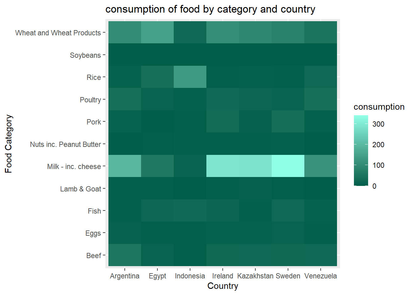
Is It Helpful??
Yes! for the right type of data, this is a helpful visual representation, and is well suited for looking at possible patterns within the data. For example we can see that the category “Milk -inc. cheese” is a highly consumed category for most of our countries represented.