tidyr::drop_na()
Amy Olyaei
In this document, I will introduce the drop_na() function and show what it’s for.
#load tidyr up
library(tidyverse)
## Warning: package 'tidyverse' was built under R version 4.0.3## -- Attaching packages --------------------------------------- tidyverse 1.3.0 --## v ggplot2 3.3.3 v purrr 0.3.4
## v tibble 3.0.6 v dplyr 1.0.4
## v tidyr 1.1.2 v stringr 1.4.0
## v readr 1.4.0 v forcats 0.5.1## Warning: package 'ggplot2' was built under R version 4.0.3## Warning: package 'tibble' was built under R version 4.0.3## Warning: package 'tidyr' was built under R version 4.0.3## Warning: package 'readr' was built under R version 4.0.3## Warning: package 'purrr' was built under R version 4.0.3## Warning: package 'dplyr' was built under R version 4.0.3## Warning: package 'stringr' was built under R version 4.0.3## Warning: package 'forcats' was built under R version 4.0.3## -- Conflicts ------------------------------------------ tidyverse_conflicts() --
## x dplyr::filter() masks stats::filter()
## x dplyr::lag() masks stats::lag()library(tidyr)
library(dplyr)
#example dataset
library(palmerpenguins)## Warning: package 'palmerpenguins' was built under R version 4.0.3data(penguins)What is it for?
The drop_na() function accepts two arguments: the first is the dataset, and the second is ... which is the columns you want to inspect for missing values. The second argument makes this function most appropriately used within a tidy workflow and essential when wanting to specify for a specific column.
Within this first example, we can see how to use the function within a tidy workflow. The drop_na() is removing rows from the data set based off the ‘NA’ arguments within the sex column. As one can see, the original tibble contained 12 rows; however, after applying the function it only contains 7 rows.
#Slicing the data
penguins%>%
  slice(1:12)
## # A tibble: 12 x 8
## species island bill_length_mm bill_depth_mm flipper_length_~ body_mass_g
## <fct> <fct> <dbl> <dbl> <int> <int>
## 1 Adelie Torge~ 39.1 18.7 181 3750
## 2 Adelie Torge~ 39.5 17.4 186 3800
## 3 Adelie Torge~ 40.3 18 195 3250
## 4 Adelie Torge~ NA NA NA NA
## 5 Adelie Torge~ 36.7 19.3 193 3450
## 6 Adelie Torge~ 39.3 20.6 190 3650
## 7 Adelie Torge~ 38.9 17.8 181 3625
## 8 Adelie Torge~ 39.2 19.6 195 4675
## 9 Adelie Torge~ 34.1 18.1 193 3475
## 10 Adelie Torge~ 42 20.2 190 4250
## 11 Adelie Torge~ 37.8 17.1 186 3300
## 12 Adelie Torge~ 37.8 17.3 180 3700
## # ... with 2 more variables: sex <fct>, year <int>#Dropping based on sex
penguins%>%
slice(1:12) %>%
drop_na(sex)## # A tibble: 7 x 8
## species island bill_length_mm bill_depth_mm flipper_length_~ body_mass_g sex
## <fct> <fct> <dbl> <dbl> <int> <int> <fct>
## 1 Adelie Torge~ 39.1 18.7 181 3750 male
## 2 Adelie Torge~ 39.5 17.4 186 3800 fema~
## 3 Adelie Torge~ 40.3 18 195 3250 fema~
## 4 Adelie Torge~ 36.7 19.3 193 3450 fema~
## 5 Adelie Torge~ 39.3 20.6 190 3650 male
## 6 Adelie Torge~ 38.9 17.8 181 3625 fema~
## 7 Adelie Torge~ 39.2 19.6 195 4675 male
## # ... with 1 more variable: year <int>Within the second examples, we can see that without specifying by a column all rows containing ‘NA’ will be removed from the data set. I chose to use a tidy work flow in this example so the removing of the rows could be easily visualized; however, if the ultimate desire is to remove all the ‘NA’ arguments from the data one could simply go ‘drop_na(dataset)’.
#Dropping all Na variables
penguins%>%
  slice(1:12) %>%
  drop_na()
## # A tibble: 7 x 8
## species island bill_length_mm bill_depth_mm flipper_length_~ body_mass_g sex
## <fct> <fct> <dbl> <dbl> <int> <int> <fct>
## 1 Adelie Torge~ 39.1 18.7 181 3750 male
## 2 Adelie Torge~ 39.5 17.4 186 3800 fema~
## 3 Adelie Torge~ 40.3 18 195 3250 fema~
## 4 Adelie Torge~ 36.7 19.3 193 3450 fema~
## 5 Adelie Torge~ 39.3 20.6 190 3650 male
## 6 Adelie Torge~ 38.9 17.8 181 3625 fema~
## 7 Adelie Torge~ 39.2 19.6 195 4675 male
## # ... with 1 more variable: year <int>Additionally, the drop_na() function is useful when plotting data. When the ‘drop_na()’ function is not applied to the tidy workflow one can see that the ‘NA’ values are treated as a category within the sex column. However, when drop_na() is included the values are removed providing a better display of the data.
#Using in graph pipe
library(ggplot2)

#Keeping the NA values of sex within the graphical display
penguins %>%
  count(sex, species) %>%
  ggplot() + geom_col(aes(x = species, y = n, fill = species)) +
facet_wrap(~sex) 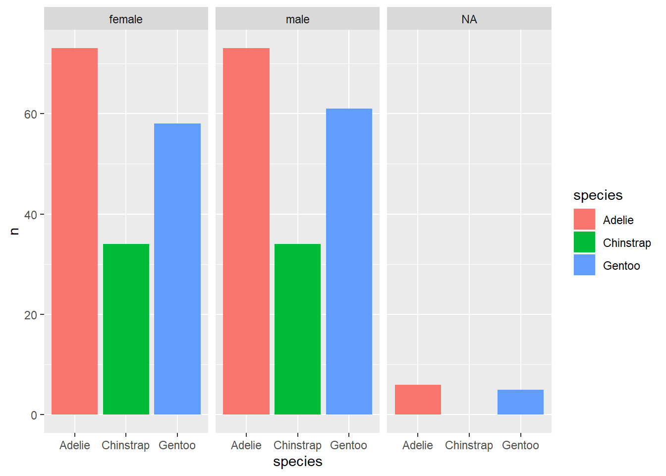
#Removing the NA values of sex within the graphical display
penguins %>%
  drop_na() %>%
  count(sex, species) %>%
  ggplot() + geom_col(aes(x = species, y = n, fill = species)) +
facet_wrap(~sex) 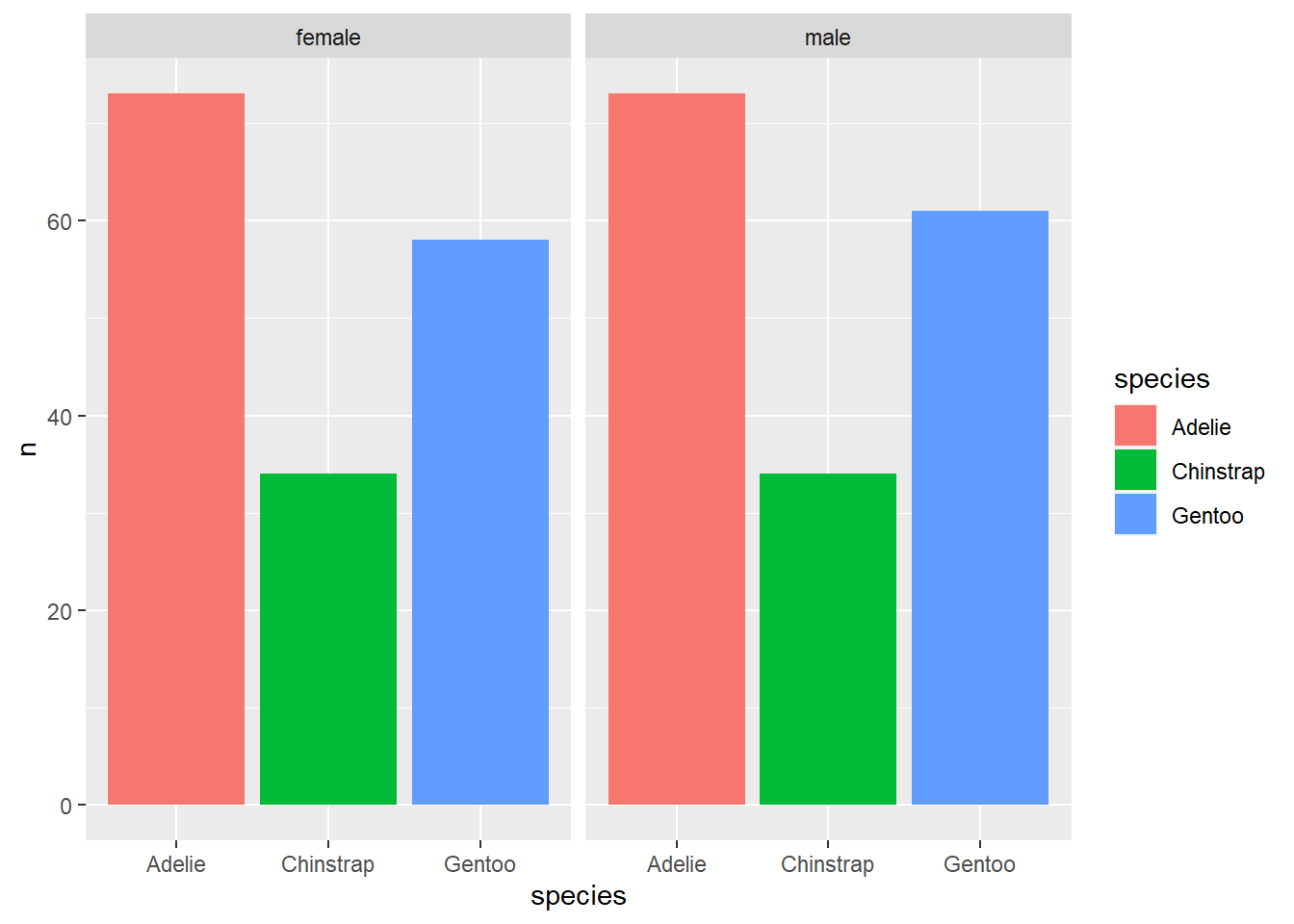
Is it helpful?
Yes, I believe this function is helpful especially if you want to remove missing values from only a specific column.